Randomized algorithms are hard to test. Their outputs are, by design, unpredictable—and that unpredictability is a feature, not a bug. It is what gives them useful guarantees like unbiasedness and computational efficiency. But it also makes them slippery: how do you check that a stochastic program is correct when it gives different answers every time you run it?
This post sketches some ideas for how to think about testing randomized algorithms—especially the kinds of algorithms that we use for probabilistic inference. I'll present a concrete sampling algorithm with several plausible implementations—some correct, some subtly broken—and develop progressively more powerful testing strategies to tell them apart.
A Tricky Little Sampling Algorithm
Suppose we have a distribution $p$ over a finite set $\mathcal{X} = \{1, \ldots, N\}$ and a condition $C \subseteq \mathcal{X}$ (the set of "good" elements). We want to sample from the conditional distribution $p(\cdot \mid C)$. But rather than returning a plain sample, we want a properly weighted sample $(x, w)$—a sample-weight pair that can be used for unbiased estimation.
The following algorithm, which we call AWRS (from Lipkin et al., 2025), does exactly this. Here is the pseudocode from the paper:
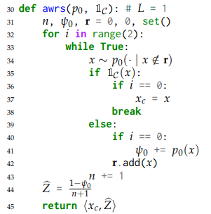
The idea: run rejection sampling twice. The first pass finds a conditioned sample $x^*$ while tracking the total rejected probability mass $\psi$. The second pass generates additional rejections to get a count $n$. The weight $(1 - \psi) / (n + 1)$ combines these two signals—the rejected mass and the rejection count—into an unbiased estimate of the normalizing constant $Z$. The number of rejections before finding a valid token contains signal about the magnitude of $Z$, and weighting by the actual probability mass removed (rather than just counting) reduces variance.
Four Implementations, at Least One Bug
Did we implement it correctly? That's the question we'd like our tests to answer. To make the exercise concrete, here are four Python implementations. They all look reasonable, but at least one has a bug. Which ones are correct?
Each variant takes a draw parameter that defaults to sampling from a
categorical distribution. This is a hook we'll exploit later: in production it
calls the RNG, but in testing we'll swap it for something that lets us
enumerate every possible execution.
Variant A
def awrs_a(p, cond, draw=sample_categorical):
    p_cond = p.copy()
    n, psi = 0, 0
    xc0 = None
    for i in range(2):
        while True:
            x = draw(p_cond / p_cond.sum(), context=('awrs', i, xc0))
            if cond(x):
                if i == 0:
                    xc0 = x
                break
            else:
                if i == 0:
                    psi += p_cond[x]
                p_cond[x] = 0
            n += 1
    return xc0, (1 - psi) / (n + 1)
Variant B
def awrs_b(p, cond, draw=sample_categorical):
    p_cond = p.copy()
    n, psi = 0, 0
    xc0 = None
    for i in range(2):
        while True:
            x = draw(p_cond / p_cond.sum(), context=('awrs', i, xc0))
            if cond(x):
                if i == 0:
                    xc0 = x
                break
            else:
                if i == 0:
                    psi += p_cond[x]
                p_cond[x] = 0
            n += 1
    return xc0, (1 + psi) / (n + 1)
Variant C
def awrs_c(p, cond, draw=sample_categorical):
    p_cond = p.copy()
    n, psi = 0, 0
    xc0 = None
    for i in range(2):
        while True:
            x = draw(p_cond / p_cond.sum(), context=('awrs', i, xc0))
            if cond(x):
                if i == 0:
                    xc0 = x
                break
            else:
                psi += p_cond[x]
                p_cond[x] = 0
            n += 1
    return xc0, (1 - psi) / (n + 1)
Variant D
def awrs_d(p, cond, draw=sample_categorical):
    p_cond = p.copy()
    n, psi = 0, 0
    xc0 = None
    for i in range(2):
        while True:
            x = draw(p_cond / p_cond.sum(), context=('awrs', i, xc0))
            if cond(x):
                if i == 0:
                    xc0 = x
                break
            else:
                if i == 0:
                    psi += p_cond[x]
                p_cond[x] = 0
            n += 1
    return xc0, (1 - psi) / (n + 2)
Each variant differs from the others by a single line. I encourage you to read them carefully and try to spot the differences before scrolling further.
Hint
Compare the else branch and the return statement across the four variants.
Our job is to build testing strategies that catch the buggy ones—ideally without needing to know which line is wrong.
But before we can test anything, we need to answer the most important question in all of software testing:
What Should This Code Do?
You cannot test code without a specification. For randomized algorithms, the specification comes from theory—and translating theory into a checkable property is half the battle. We'll keep coming back to this question for every algorithm in this post.
For AWRS, the specification is: it should return a sample-weight pair $(x, w)$ such that $w \cdot \mathbf{1}[x = x']$ is an unbiased estimator of the unnormalized conditional distribution for every $x' \in \mathcal{X}$:
$$ \mathop{\mathbb{E}}_{(x,w) \sim \text{AWRS}} \left[ w \cdot \mathbf{1}[x = x'] \right] = p(x') \cdot \mathbf{1}[x' \in C] $$
The right-hand side is the unnormalized target—$p$ restricted to the condition $C$, with normalizing constant $Z = \sum_{x \in C} p(x)$.
Note that you may often need to tweak definitions, narrow or broaden the scope of theory in order to suit your code's intended use cases. This is an important skill for turning theory into tests.
Setting Up a Test Case
Now that we have a testable definition, we need to think about which things in the equation we can compute and which things we need to estimate. Let's make a concrete test case:
np.random.seed(0)
N = 4
p = np.random.dirichlet(np.ones(N))  # random distribution over {0,...,N-1}
cond = np.random.uniform(0, 1, size=N) < 0.5  # random subset

Z = p[cond].sum()
target = p * cond  # unnormalized target (not a distribution!)
Strategy 1: Monte Carlo Averaging
The obvious first testing strategy: run the code "a lot of times" and compute an average.
np.random.seed(0)
reps = 1_000
for name, awrs in variants.items():
    have = np.zeros(N)
    for r in range(1, 1 + reps):
        (x, w) = awrs(p, lambda x: cond[x])
        have[x] += w
    err = abs(have / reps - target).sum()
    print(f'Variant {name}: error = {err:.6f}')
Variant A: error = 0.025367
Variant B: error = 0.163426
Variant C: error = 0.051898
Variant D: error = 0.173738
Is this error small enough? How do you know?
This is the central problem with Monte Carlo testing: a single number tells you almost nothing without a reference frame. We need to know what should happen as we increase the number of samples.
Convergence Rates
A better approach is to watch the error decrease as a function of the number of samples $M$. It should keep going down forever, modulo numerical precision. And crucially, we often know the rate at which it should decrease.
The general picture: suppose we have a sequence of estimators $\widehat{\mu}^{(M)}$ targeting some quantity $\mu$. The mean squared error decomposes as
$$ \mathop{\mathbb{E}} \| \widehat{\mu}^{(M)} - \mu \|^2 = \| \mathop{\mathbb{E}}[\widehat{\mu}^{(M)}] - \mu \|^2 + \mathop{\mathbb{E}} \| \widehat{\mu}^{(M)} - \mathop{\mathbb{E}}[\widehat{\mu}^{(M)}] \|^2 $$
The first term is the squared bias; the second is the variance (more precisely, the trace of the covariance of $\widehat{\mu}^{(M)}$). Different classes of estimators make different predictions about how these terms behave:
-
I.I.D. unbiased (e.g., our AWRS test). The bias is zero for all $M$. The variance is $V/M$ where $V = \text{tr}(\text{Cov}(X))$—the sum of the componentwise variances of a single sample. So $\mathop{\mathbb{E}} \| \widehat{\mu}^{(M)} - \mu \|^2 = V/M$.If you prefer root mean squared error, the slope is $-1/2$ and the intercept is $\frac{1}{2} \log V$.
-
Correlated but unbiased (e.g., MCMC, Markov reward processes). The bias is still zero, but autocorrelation inflates the variance: $\mathop{\mathbb{E}} \| \widehat{\mu}^{(M)} - \mu \|^2 \approx V_{\text{eff}} / M$ where $V_{\text{eff}} > V$ depends on the integrated autocorrelation time. The rate is still $O(1/M)$, but the constant is larger.
-
Biased but consistent (e.g., self-normalized importance sampling). The bias is $O(1/M)$, so $\| \mathop{\mathbb{E}}[\widehat{\mu}^{(M)}] - \mu \|^2 = O(1/M^2)$. The variance is $O(1/M)$. The MSE is still $O(1/M)$ overall, so on a log–log plot the slope looks the same—the bias hides in the noise at large $M$.
In all three cases, $\text{MSE} \sim c / M$ for some constant $c$, which means $\log \text{MSE} = -\log M + \log c$: a line with slope $-1$ on a log–log plot. The intercept $\log c$ tells us the constant.
Deriving $\,V\,$ for vector-valued estimators
Our estimator is vector-valued (a distribution over $N$ elements), so we need a scalar measure of error. The natural choice is the squared $L_2$ norm $\| \widehat{\mu}^{(M)} - \mu \|^2$ where $\widehat{\mu}^{(M)} = \frac{1}{M} \sum_{m=1}^{M} X^{(m)}$ and $\mu = \mathop{\mathbb{E}}[X^{(m)}]$:
$$ \mathop{\mathbb{E}} \| \widehat{\mu}^{(M)} - \mu \|^2 = \mathop{\mathbb{E}} \sum_{j=1}^{N} (\widehat{\mu}^{(M)}_j - \mu_j)^2 = \sum_{j=1}^{N} \text{Var}(\widehat{\mu}^{(M)}_j) = \frac{1}{M} \sum_{j=1}^{N} \text{Var}(X^{(m)}_j) = \frac{V}{M} $$
where $V = \text{tr}(\text{Cov}(X^{(m)}))$ is the trace of the covariance matrix of a single sample. The last step uses independence; for correlated samples, the $1/M$ factor becomes $1/M$ times an autocorrelation correction.
fig, axes = plt.subplots(2, 2, figsize=(10, 7), sharex=True, sharey=True)

for ax, (name, awrs) in zip(axes.flat, variants.items()):
    np.random.seed(0)
    M = 10_000
    have = np.zeros(N)
    xs, ys = [], []
    for r in range(1, 1 + M):
        (item, w) = awrs(p, lambda x: cond[x])
        have[item] += w
        if r >= 20:
            xs.append(r)
            ys.append(abs(have / r - target).sum())
    slope, intercept = np.polyfit(np.log(xs), np.log(ys), deg=1)
    ax.plot(xs, ys, alpha=0.7, lw=0.8)
    ax.plot(xs, np.exp(np.log(xs) * slope + intercept), c='r', lw=2,
            label=f'slope = {slope:.2f}')
    ax.set_xscale('log'); ax.set_yscale('log')
    ax.set_title(f'Variant {name}')
    ax.legend(fontsize=9)

axes[1,0].set_xlabel('number of samples')
axes[1,1].set_xlabel('number of samples')
axes[0,0].set_ylabel('error')
axes[1,0].set_ylabel('error')
fig.tight_layout()
plt.show()

A note on reading this plot: when we say "log–log scale" we mean the axes are
log-transformed but the tick labels show the original values (e.g., $10^2$,
$10^3$). This is what plt.xscale('log') does. This is different from
literally plotting $\log y$ vs $\log x$, where the axes are linear but the
values are logs. The line-fitting code does the latter ($\texttt{np.polyfit}$ on
$\log x$, $\log y$), but for visual inspection, log-scaled axes are usually
clearer because you can read off the original quantities directly.
The fitted slope should be close to $-0.5$ (we're plotting error, not squared error), which is exactly what we see.
What a Single Run Can and Can't Tell Us
Watching a single long run tells us the rate of convergence, but it can't distinguish the three cases above. An unbiased i.i.d. estimator, a correlated MCMC chain, and a self-normalized importance sampler can all produce very similar log–log plots—the slopes are the same and the constants differ in ways that are hard to eyeball.
A pedagogical example: suppose we accidentally computed the average as $\frac{1}{M+1} \sum_{m=1}^{M} X^{(m)}$ instead of $\frac{1}{M} \sum_{m=1}^{M} X^{(m)}$. This estimator is biased—it systematically underestimates the target—but consistent, because the bias factor $M/(M+1) \to 1$. The single-run convergence plot would look nearly identical.
Averaging Over Multiple Runs
To separate bias from variance, we need multiple independent runs. The idea: run the estimator many times at each sample size $M$, and compare the average behavior to the theoretical prediction.
Recall the decomposition from earlier: $\mathop{\mathbb{E}} \| \widehat{\mu}^{(M)} - \mu \|^2 = \| \mathop{\mathbb{E}}[\widehat{\mu}^{(M)}] - \mu \|^2 + \mathop{\mathbb{E}} \| \widehat{\mu}^{(M)} - \mathop{\mathbb{E}}[\widehat{\mu}^{(M)}] \|^2$. For the i.i.d. unbiased case, the variance term is $V/M$. So:
- If the observed MSE matches $V/M$, the squared bias must be near zero—evidence of unbiasedness.
- If the estimator has persistent bias, $\| \mathop{\mathbb{E}}[\widehat{\mu}^{(M)}] - \mu \|^2$ does not vanish with $M$. At large $M$, the variance $V/M$ shrinks but the bias dominates, causing the observed curve to flatten out above the theoretical line.
- For biased-but-consistent estimators (like self-normalized IS), $\| \mathop{\mathbb{E}}[\widehat{\mu}^{(M)}] - \mu \|^2 = O(1/M^2)$—it vanishes faster than the variance. This means the MSE curve will eventually match $V/M$, but may sit slightly above it for small $M$.
from scipy import stats

def mean_confidence_interval(data, confidence=0.95):
    n = len(data)
    m = np.mean(data)
    se = stats.sem(data)
    h = se * stats.t.ppf((1 + confidence) / 2, n - 1)
    return m, m - h, m + h

fig, axes = plt.subplots(2, 2, figsize=(10, 7), sharex=True, sharey=True)

for ax, (name, awrs) in zip(axes.flat, variants.items()):
    np.random.seed(0)
    reps = 1000
    M = 50
    ms = list(range(1, 1 + M))
    runs_ys = []
    samples = []
    for r in range(1, 1 + reps):
        ys = []
        have = np.zeros(N)
        for m in ms:
            (item, w) = awrs(p, lambda x: cond[x])
            have[item] += w
            onehot = np.zeros(N)
            onehot[item] = w
            samples.append(onehot)
            ys.append(np.linalg.norm(have / m - target)**2)
        runs_ys.append(ys)
    runs_ys = np.array(runs_ys)
    C = np.cov(np.array(samples).T)
    V = np.trace(C)
    cis = [mean_confidence_interval(runs_ys[:, m]) for m in range(M)]
    means = [x[0] for x in cis]
    lowers = [x[1] for x in cis]
    uppers = [x[2] for x in cis]
    ax.plot(ms, means, c='b', label='observed')
    ax.fill_between(ms, lowers, uppers, alpha=0.2, color='b')
    ax.plot(ms, V / np.array(ms), label='theoretical',
            c='orange', zorder=10, lw=2, linestyle=':')
    ax.set_title(f'Variant {name}')
    ax.set_xscale('log'); ax.set_yscale('log')
    ax.legend(fontsize=9)

axes[1,0].set_xlabel(r'number of samples ($M$)')
axes[1,1].set_xlabel(r'number of samples ($M$)')
axes[0,0].set_ylabel('mean squared error')
axes[1,0].set_ylabel('mean squared error')
fig.tight_layout()
plt.show()

The observed curve hugs the theoretical $V/M$ line, which is strong evidence that our sampler is properly weighted—not just consistent, but unbiased, with the right variance.
But Monte Carlo testing is still a blunt instrument. Small biases hide easily in the noise, and you need many runs to have any statistical power. For correlated estimators, the effective variance $V_{\text{eff}}$ may be hard to compute, making the theoretical line itself uncertain. In software—unlike the real world—we can almost always do better.
Strategy 2: Program Tracing
Here's the key insight: if the state space is small enough, we can enumerate all possible executions of the randomized program and verify the correctness condition exactly (up to floating point).
The idea is to hijack the random number generation inside the program to make it systematically explore every possible branch. We track each execution trace's probability, and combine all traces to compute the exact output distribution.
The Tracer
The implementation uses a trie data structure that mirrors the branching structure of the program's random choices. Each node in the trie corresponds to a decision point, and its children correspond to the possible outcomes.
The beautiful thing about TraceSWOR is that it works as a context manager:
each with tracer: block explores one trace, and when it exits, that trace's
mass is zeroed out so we never revisit it. We loop until the root's mass hits
zero—meaning we've exhausted every possible execution.
Tracer implementation
class Node:
    """A node in the execution trie."""
    def __init__(self, idx, mass, parent, token=None):
        self.idx = idx
        self.mass = mass          # remaining probability mass
        self.parent = parent
        self.token = token        # label for visualization
        self.child_masses = None  # set on first visit
        self.active_children = {}
        self._mass = mass         # remember original mass
        self.context = None

    def sample(self):
        """Sample a child proportional to remaining mass."""
        p = self.child_masses / self.child_masses.sum()
        return np.random.choice(len(p), p=p)

    def update(self):
        """Propagate mass changes up to the root."""
        if self.parent is not None:
            self.parent.child_masses[self.idx] = self.mass
            self.parent.mass = np.sum(self.parent.child_masses)
            self.parent.update()


class Tracer:
    """
    Lazily materializes the probability tree of a generative process
    by program tracing. Works with both array-valued and dict-valued
    distributions.
    """
    def __init__(self):
        self.root = Node(idx=-1, mass=1.0, parent=None)
        self.cur = None

    def __call__(self, p, context=None):
        """Drop-in replacement for any sampling function."""
        if isinstance(p, dict):
            keys = list(p.keys())
            vals = np.array([p[k] for k in keys])
        else:
            p = np.asarray(p, dtype=float)
            keys = list(range(len(p)))
            vals = p
        vals = vals / vals.sum()
        cur = self.cur

        if cur.child_masses is None:
            cur.child_masses = cur.mass * vals
            cur.context = context

        a = cur.sample()
        if a not in cur.active_children:
            cur.active_children[a] = Node(
                idx=a, mass=cur.child_masses[a], parent=cur,
                token=keys[a],
            )
        self.cur = cur.active_children[a]
        return keys[a]


class TraceSWOR(Tracer):
    """
    Sampling without replacement meets program tracing.

    Each execution trace is explored exactly once. After a trace
    completes, its probability mass is zeroed out and propagated
    up the trie, ensuring the next trace is fresh.
    """
    def __enter__(self):
        self.cur = self.root

    def __exit__(self, *args):
        self.cur.mass = 0
        self.cur.update()
Exact Verification
Now we can verify all four AWRS variants exactly:
import html as html_module
from graphviz import Digraph

class Node:
    def __init__(self, idx, mass, parent, token=None):
        self.idx = idx
        self.mass = mass
        self.parent = parent
        self.token = token
        self.child_masses = None
        self.active_children = {}
        self._mass = mass
        self.context = None

    def sample(self):
        cm = self.child_masses
        p = cm / cm.sum()
        return np.random.choice(len(p), p=p)

    def update(self):
        if self.parent is not None:
            self.parent.child_masses[self.idx] = self.mass
            self.parent.mass = np.sum(self.parent.child_masses)
            self.parent.update()

    def graphviz(self):
        g = Digraph(
            graph_attr=dict(rankdir='LR'),
            node_attr=dict(fontname='Monospace', fontsize='10',
                           height='.05', width='.05', margin='0.055,0.042'),
            edge_attr=dict(arrowsize='0.3', fontname='Monospace', fontsize='9'),
        )
        counter = [0]
        ids = {}
        def get_id(node):
            if id(node) not in ids:
                ids[id(node)] = str(counter[0])
                counter[0] += 1
            return ids[id(node)]
        q = [self]
        visited = set()
        while q:
            x = q.pop()
            if id(x) in visited: continue
            visited.add(id(x))
            label = ''
            if x.context:
                label += f'{x.context}\n'
            label += f'{x._mass:.2g}'
            g.node(get_id(x), label=label, shape='box')
            if x.child_masses is not None:
                for a, y in x.active_children.items():
                    tok = y.token if y.token is not None else a
                    edge_label = f'{html_module.escape(str(tok))}/{y._mass/x._mass:.2g}'
                    g.edge(get_id(x), get_id(y), label=edge_label)
                    q.append(y)
        return g

class Tracer:
    def __init__(self):
        self.root = Node(idx=-1, mass=1.0, parent=None)
        self.cur = None

    def __call__(self, p, context=None):
        if isinstance(p, dict):
            keys = list(p.keys())
            vals = np.array([p[k] for k in keys])
        else:
            p = np.asarray(p, dtype=float)
            keys = list(range(len(p)))
            vals = p
        vals = vals / vals.sum()
        cur = self.cur
        if cur.child_masses is None:
            cur.child_masses = cur.mass * vals
            cur.context = context
        a = cur.sample()
        if a not in cur.active_children:
            cur.active_children[a] = Node(
                idx=a, mass=cur.child_masses[a], parent=cur, token=keys[a])
        self.cur = cur.active_children[a]
        return keys[a]

class TraceSWOR(Tracer):
    def __enter__(self):
        self.cur = self.root
    def __exit__(self, *args):
        self.cur.mass = 0
        self.cur.update()

# Exact verification for all variants
for name, awrs in variants.items():
    tracer = TraceSWOR()
    prob = np.zeros(N)
    while tracer.root.mass > 0:
        with tracer:
            (item, w) = awrs(p, lambda x: cond[x], draw=tracer)
            prob[item] += w * tracer.cur.mass
    err = abs(target - prob).sum()
    status = '\u2713' if np.allclose(target, prob) else '\u2717'
    print(f'Variant {name}: {status}  (error = {err:.2e})')
Variant A: ✓  (error = 5.55e-17)
Variant B: ✗  (error = 1.60e-01)
Variant C: ✗  (error = 4.99e-02)
Variant D: ✗  (error = 1.80e-01)
This is not a statistical test. It is an exact check (modulo floating point) that the proper weighting condition holds. No confidence intervals, no squinting at log–log plots. The tracer gives a definitive yes or no for each variant.
The difference between target and prob is not zero—it rarely will be with floating point numbers. But np.allclose checks that they agree to within a reasonable tolerance ($\approx 10^{-8}$).
Strategy 3: Testing Sequential Algorithms
Program tracing is not limited to simple sampling algorithms. It works on anything that makes discrete random choices through a hookable interface. Let's apply it to sequential importance sampling (SIS) and sequential importance resampling (SIR).
Setup: Target and Proposal
SIS and SIR require two things: a target distribution $p$ and a proposal
distribution $q$, both with incremental interfaces. We sample sequences from
$q$ and reweight by $p/q$ at each step to correct for the mismatch. Both are
implemented with the same SimpleLM class, which maps prefixes to next-token
distributions via p_next.
p = SimpleLM({('a', 'a'): 0.3, ('b', 'b', 'b'): 0.6, (): 0.1})
q = SimpleLM({('a', 'a'): 0.2, ('b', 'b', 'b'): 0.7, (): 0.1})
Utilities: SimpleLM, sample_dict
EOS = '<EOS>'  # end-of-sequence marker

class SimpleLM:
    """
    A simple sequence model defined by a probabilistic context-free grammar.
    Maps prefixes to next-token distributions (as dicts).
    """
    def __init__(self, sequences):
        """
        sequences: dict mapping tuple-of-tokens to probability.
        E.g., {('a','a'): 0.3, ('b','b','b'): 0.6, (): 0.1}
        """
        self.sequences = sequences

    def p_next(self, prefix):
        """Return conditional distribution over next token given prefix."""
        dist = {}
        for seq, prob in self.sequences.items():
            if len(seq) < len(prefix):
                continue
            if seq[:len(prefix)] != prefix:
                continue
            if len(seq) == len(prefix):
                dist[EOS] = dist.get(EOS, 0) + prob
            else:
                token = seq[len(prefix)]
                dist[token] = dist.get(token, 0) + prob
        total = sum(dist.values())
        return {k: v / total for k, v in dist.items()}

def sample_dict(d, context=None):
    """Sample a key from a dict-valued distribution."""
    keys = list(d.keys())
    vals = np.array([d[k] for k in keys])
    vals = vals / vals.sum()
    idx = np.random.choice(len(keys), p=vals)
    return keys[idx]
Sequential Importance Sampling
Again: what should this code do? SIS should produce weighted particles whose weights are unbiased estimates of the normalizing constant $Z = \sum_{\mathbf{x}} p(\mathbf{x})$. Specifically, $\frac{1}{M} \sum_m w_m$ should be an unbiased estimate of $Z$—in this case, $Z = 1$ since our target is a proper distribution.
At each step, SIS extends each particle by sampling from the proposal $q$ and reweighting by $p/q$:
from collections import namedtuple
Particle = namedtuple('Particle', 'weight, string')

def sequential_importance_sampling(p, q, M, draw=sample_dict):
    unfinished = [Particle(1, ()) for _ in range(M)]
    finished = []
    while unfinished:
        next_unfinished = []
        for particle in unfinished:
            P = p.p_next(particle.string)
            Q = q.p_next(particle.string)
            x = draw(Q)
            if x == EOS:
                finished.append(Particle(
                    particle.weight * P[x] / Q[x], particle.string))
            else:
                next_unfinished.append(Particle(
                    particle.weight * P[x] / Q[x],
                    particle.string + (x,)))
        unfinished = next_unfinished
    return finished
Since our Tracer handles both arrays and dicts, the same TraceSWOR works
here without modification. Here is the trace tree for SIS:
from collections import namedtuple

EOS = '<EOS>'

class SimpleLM:
    def __init__(self, sequences):
        self.sequences = sequences
    def p_next(self, prefix):
        dist = {}
        for seq, prob in self.sequences.items():
            if len(seq) < len(prefix): continue
            if seq[:len(prefix)] != prefix: continue
            if len(seq) == len(prefix):
                dist[EOS] = dist.get(EOS, 0) + prob
            else:
                token = seq[len(prefix)]
                dist[token] = dist.get(token, 0) + prob
        total = sum(dist.values())
        return {k: v / total for k, v in dist.items()}

Particle = namedtuple('Particle', 'weight, string')

def sequential_importance_sampling(p, q, M, draw):
    unfinished = [Particle(1, ()) for _ in range(M)]
    finished = []
    while unfinished:
        next_unfinished = []
        for particle in unfinished:
            P = p.p_next(particle.string)
            Q = q.p_next(particle.string)
            x = draw(Q)
            if x == EOS:
                finished.append(Particle(particle.weight * P[x] / Q[x], particle.string))
            else:
                next_unfinished.append(Particle(particle.weight * P[x] / Q[x], particle.string + (x,)))
        unfinished = next_unfinished
    return finished

p_lm = SimpleLM({('a', 'a'): 0.3, ('b', 'b', 'b'): 0.6, (): 0.1})
q_lm = SimpleLM({('a', 'a'): 0.2, ('b', 'b', 'b'): 0.7, (): 0.1})

tracer = TraceSWOR()
have = 0
while tracer.root.mass > 0:
    with tracer:
        finished = sequential_importance_sampling(p_lm, q_lm, M=1, draw=tracer)
        Z_hat = sum(pt.weight for pt in finished)
        have += Z_hat * tracer.cur.mass

print(f'Z estimate (exact via tracing): {have:.6f}')
print(f'Z true:                         1.000000')
assert abs(have - 1.0) < 1e-10
print('\u2713 SIS is unbiased')
tracer.root.graphviz()
Z estimate (exact via tracing): 1.000000
Z true:                         1.000000
✓ SIS is unbiased

Sequential Importance Resampling
What should this code do? The same thing as SIS—produce an unbiased estimate of $Z$—but with lower variance via adaptive resampling.
SIR adds a resampling step when the effective sample size drops below a threshold. This creates more diverse particles but also more execution traces:
def sequential_importance_resampling(p, q, M, tau, draw=sample_dict):
    unfinished = [Particle(1, ()) for _ in range(M)]
    finished = []
    t = 0
    while True:
        t += 1
        next_unfinished = []
        for m, particle in enumerate(unfinished):
            P = p.p_next(particle.string)
            Q = q.p_next(particle.string)
            x = draw(Q, context=(t, m))
            if x == EOS:
                finished.append(Particle(
                    particle.weight * P[x] / Q[x], particle.string))
            else:
                next_unfinished.append(Particle(
                    particle.weight * P[x] / Q[x],
                    particle.string + (x,)))
        unfinished = next_unfinished
        if not unfinished:
            break

        W = sum(particle.weight for particle in unfinished)
        W2 = sum(particle.weight**2 for particle in unfinished)
        M_eff = W**2 / W2

        if M_eff < tau * M:
            distr = {k: particle.weight / W
                     for k, particle in enumerate(unfinished)}
            indices = [draw(distr, context=('resample', t, m))
                       for m in range(M)]
            avg_weight = W / M
            unfinished = [Particle(avg_weight, unfinished[k].string)
                          for k in indices]

    return finished
Here is the trace tree for SIR—notice that with resampling we have more traces than without. This is because there are more places that request random decisions in the code.
def sequential_importance_resampling(p, q, M, tau, draw):
    unfinished = [Particle(1, ()) for _ in range(M)]
    finished = []
    t = 0
    while True:
        t += 1
        next_unfinished = []
        for m, particle in enumerate(unfinished):
            P = p.p_next(particle.string)
            Q = q.p_next(particle.string)
            x = draw(Q, context=(t, m))
            if x == EOS:
                finished.append(Particle(particle.weight * P[x] / Q[x], particle.string))
            else:
                next_unfinished.append(Particle(particle.weight * P[x] / Q[x], particle.string + (x,)))
        unfinished = next_unfinished
        if not unfinished: break
        W = sum(pt.weight for pt in unfinished)
        W2 = sum(pt.weight**2 for pt in unfinished)
        M_eff = W**2 / W2
        if M_eff < tau * M:
            distr = {k: pt.weight / W for k, pt in enumerate(unfinished)}
            indices = [draw(distr, context=('resample', t, m)) for m in range(M)]
            avg_weight = W / M
            unfinished = [Particle(avg_weight, unfinished[k].string) for k in indices]
    return finished

tracer = TraceSWOR()
have = 0
while tracer.root.mass > 0:
    with tracer:
        finished = sequential_importance_resampling(p_lm, q_lm, tau=0.75, M=3, draw=tracer)
        Z_hat = sum(pt.weight for pt in finished) / 3
        have += Z_hat * tracer.cur.mass

print(f'Z estimate (exact via tracing): {have:.6f}')
print(f'Z true:                         1.000000')
assert abs(have - 1.0) < 1e-10
print('\u2713 SIR is unbiased')
tracer.root.graphviz()
Z estimate (exact via tracing): 1.000000
Z true:                         1.000000
✓ SIR is unbiased

Pro tip: Make sure the total mass decreases quickly, as the loop will halt only when the total mass is zero. This requires the support to be finite. For problems where the support is large but finite, it may be a reasonable heuristic to stop early if the remaining mass is small, trading exactness for an unbiased estimate (via techniques from Shi et al., 2020).Traces are a combinatorial space, so this strategy is only practical for smaller problems. But "smaller problems" is exactly the regime where tests should live—small enough to verify exactly, but complex enough to exercise the algorithm's logic.
Some Miscellaneous Thoughts
Testing is fundamentally about control. Some abstractions give us more control over a system's behavior than others, and good tests depend on choosing abstractions that make critical behaviors observable, reproducible, and manipulable.
The draw parameter in all of the algorithms above is a good example. It's a
tiny abstraction—just a function that returns a random choice—but it gives us
enormous leverage. In production, it calls the RNG. In testing, it becomes a
tracer that enumerates every possible execution. Same algorithm, radically
different observability.
A few principles I've found useful:
-
Theory gives you test cases. The proper weighting definition, the unbiasedness of importance sampling, the convergence rate of Monte Carlo—these are all specifications that can be mechanically checked. If you don't understand the theory behind your algorithm, you don't know what to test.
-
Small exact tests beat large approximate tests. A tracer that exhaustively checks a 4-element distribution is worth more than a Monte Carlo test with 10,000 samples. The tracer gives you a definitive yes/no; the Monte Carlo test gives you a squiggly line that you have to interpret.
-
Inject errors to calibrate your tests. A test that passes on correct code but also passes on buggy code is useless. Deliberately break the algorithm and verify that your test catches it.
-
Monte Carlo is the blunt instrument of last resort. It's indispensable when the state space is too large to enumerate, but in software—unlike the real world—we can almost always find ways to do better. Freezing the RNG makes your code deterministic, but it is at best a regression test and extremely brittle.
Of course, some behaviors are only visible from "1,000 feet"—via integration tests, stress tests, or long-horizon statistical checks. Not everything can be checked with a microscope. But the more control you have over the randomness in your program, the more you can check exactly rather than approximately.