KL-divergence as an objective function

It's well-known that KL-divergence is not symmetric, but which direction is right for fitting your model?

Which KL is which? A cheat sheet

If we're fitting \(q_\theta\) to \(p\) using

\(\textbf{KL}(p || q_\theta)\)

mean-seeking, inclusive (more principled because approximates the full distribution)
requires normalization wrt \(p\) (i.e., often not computationally convenient)

\(\textbf{KL}(q_\theta || p)\)

mode-seeking, exclusive
no normalization wrt \(p\) (i.e., computationally convenient)

Mnemonic: "When the truth comes first, you get the whole truth" (h/t Philip Resnik). Here "whole truth" corresponds to the inclusiveness of \(\textbf{KL}(p || q)\).

As far as remembering the equation, I pretend that "\(||\)" is a division symbol, which happens to correspond nicely to a division symbol in the equation (I'm not sure it's intentional).

Inclusive vs. exclusive divergence

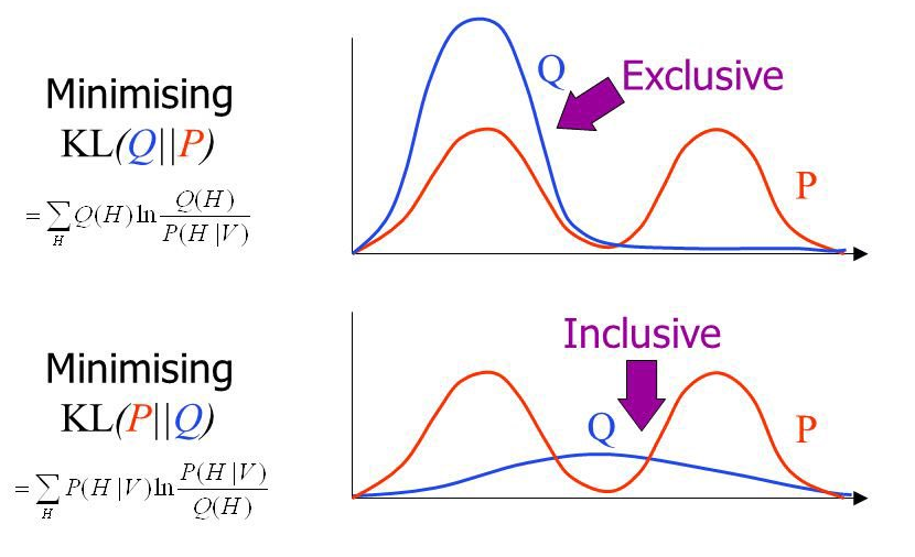Figure by John Winn.

Computational perspecive

Let's look at what's involved in fitting a model \(q_\theta\) in each direction. In this section, I'll describe the gradient and pay special attention to the issue of normalization.

Notation: \(p,q_\theta\) are probabilty distributions. \(p = \bar{p} / Z_p\), where \(Z_p\) is the normalization constant. Similarly for \(q\).

The easy direction \(\textbf{KL}(q_\theta || p)\)

\begin{align*} \textbf{KL}(q_\theta || p) &= \sum_d q(d) \log \left( \frac{q(d)}{p(d)} \right) \\ &= \sum_d q(d) \left( \log q(d) - \log p(d) \right) \\ &= \underbrace{\sum_d q(d) \log q(d)}_{-\text{entropy}} - \underbrace{\sum_d q(d) \log p(d)}_{\text{cross-entropy}} \\ \end{align*}

Let's look at normalization of \(p\), the entropy term is easy because there is no \(p\) in it.

\begin{align*} \sum_d q(d) \log p(d) &= \sum_d q(d) \log (\bar{p}(d) / Z_p) \\ &= \sum_d q(d) \left( \log \bar{p}(d) - \log Z_p) \right) \\ &= \sum_d q(d) \log \bar{p}(d) - \sum_d q(d) \log Z_p \\ &= \sum_d q(d) \log \bar{p}(d) - \log Z_p \end{align*}

In this case, \(-\log Z_p\) is an additive constant, which can be dropped because we're optimizing.

This leaves us with the following optimization problem:

\begin{align*} & \underset{\theta}{\text{argmin}}\, \textbf{KL}(q_\theta || p) \\ &\qquad = \underset{\theta}{\text{argmin}}\, \sum_d q_\theta(d) \log q_\theta(d) - \sum_d q_\theta(d) \log \bar{p}(d) \end{align*}

Let's work out the gradient

\begin{align*} & \nabla\left[ \sum_d q_\theta(d) \log q_\theta(d) - \sum_d q_\theta(d) \log \bar{p}(d) \right] \\ &\qquad = \sum_d \nabla \left[ q_\theta(d) \log q_\theta(d) \right] - \sum_d \nabla\left[ q_\theta(d) \right] \log \bar{p}(d) \\ &\qquad = \sum_d \nabla \left[ q_\theta(d) \right] \left( 1 + \log q_\theta(d) \right) - \sum_d \nabla\left[ q_\theta(d) \right] \log \bar{p}(d) \\ &\qquad = \sum_d \nabla \left[ q_\theta(d) \right] \left( 1 + \log q_\theta(d) - \log \bar{p}(d) \right) \\ &\qquad = \sum_d \nabla \left[ q_\theta(d) \right] \left( \log q_\theta(d) - \log \bar{p}(d) \right) \\ \end{align*}

We killed the one in the last equality because \(\sum_d \nabla \left[ q(d) \right] = \nabla \left[ \sum_d q(d) \right] = \nabla \left[ 1 \right] = 0\), for any \(q\) which is a probability distribution.

This direction is convenient because we don't need to normalize \(p\). Unfortunately, the "easy" direction is nonconvex in general—unlike the "hard" direction, which (as we'll see shortly) is convex.

Harder direction \(\textbf{KL}(p || q_\theta)\)

\begin{align*} \textbf{KL}(p || q_\theta) &= \sum_d p(d) \log \left( \frac{p(d)}{q(d)} \right) \\ &= \sum_d p(d) \left( \log p(d) - \log q(d) \right) \\ &= \sum_d p(d) \log p(d) - \sum_d p(d) \log q(d) \\ \end{align*}

Clearly the first term (entropy) won't matter if we're just trying optimize wrt \(\theta\). So, let's focus on the second term (cross-entropy).

\begin{align*} \sum_d p(d) \log q(d) &= \frac{1}{Z_p} \sum_d \bar{p}(d) \log \left( \bar{q}(d)/Z_q \right) \\ &= \frac{1}{Z_p} \sum_d \bar{p}(d) \left( \log \bar{q}(d) - \log Z_q \right) \\ &= \left(\frac{1}{Z_p} \sum_d \bar{p}(d) \log \bar{q}(d)\right) - \left(\frac{1}{Z_p} \sum_d \bar{p}(d) \log Z_q\right) \\ &= \left(\frac{1}{Z_p} \sum_d \bar{p}(d) \log \bar{q}(d)\right) - \left( \log Z_q \right) \left( \frac{1}{Z_p} \sum_d \bar{p}(d)\right) \\ &= \left(\frac{1}{Z_p} \sum_d \bar{p}(d) \log \bar{q}(d)\right) - \log Z_q \end{align*}

The gradient, when \(q\) is in the exponential family, is intuitive:

\begin{align*} \nabla \left[ \frac{1}{Z_p} \sum_d \bar{p}(d) \log \bar{q}(d) - \log Z_q \right] &= \frac{1}{Z_p} \sum_d \bar{p}(d) \nabla \left[ \log \bar{q}(d) \right] - \nabla \log Z_q \\ &= \frac{1}{Z_p} \sum_d \bar{p}(d) \phi_q(d) - \mathbb{E}_q \left[ \phi_q \right] \\ &= \mathbb{E}_p \left[ \phi_q \right] - \mathbb{E}_q \left[ \phi_q \right] \end{align*}

Why do we say this is hard to compute? Well, for most interesting models, we can't compute \(Z_p = \sum_d \bar{p}(d)\). This is because \(p\) is presumed to be a complex model (e.g., the real world, an intricate factor graph, a complicated Bayesian posterior). If we can't compute \(Z_p\), it's highly unlikely that we can compute another (nontrivial) integral under \(\bar{p}\), e.g., \(\sum_d \bar{p}(d) \log \bar{q}(d)\).

Nonetheless, optimizing KL in this direction is still useful. Examples include: expectation propagation, variational decoding, and maximum likelihood estimation. In the case of maximum likelihood estimation, \(p\) is the empirical distribution, so technically you don't have to compute its normalizing constant, but you do need samples from it, which can be just as hard to get as computing a normalization constant.

Optimization problem is convex when \(q_\theta\) is an exponential family—i.e., for any \(p\) the optimization problem is "easy." You can think of maximum likelihood estimation (MLE) as a method which minimizes KL divergence based on samples of \(p\). In this case, \(p\) is the true data distribution! The first term in the gradient is based on a sample instead of an exact estimate (often called "observed feature counts"). The downside, of course, is that computing \(\mathbb{E}_p \left[ \phi_q \right]\) might not be tractable or, for MLE, require tons of samples.

Remarks

In many ways, optimizing exclusive KL makes no sense at all! Except for the fact that it's computable when inclusive KL is often not. Exclusive KL is generally regarded as "an approximation" to inclusive KL. This bias in this approximation can be quite large.
Inclusive vs. exclusive is an important distinction: Inclusive divergences require \(q > 0\) whenever \(p > 0\) (i.e., no "false negatives"), whereas exclusive divergences favor a single mode (i.e., only a good fit around a that mode).
When \(q\) is an exponential family, \(\textbf{KL}(p || q_\theta)\) will be convex in \(\theta\), no matter how complicated \(p\) is, whereas \(\textbf{KL}(q_\theta || p)\) is generally nonconvex (e.g., if \(p\) is multimodal).
Computing the value of either KL divergence requires normalization. However, in the "easy" (exclusive) direction, we can optimize KL without computing \(Z_p\) (as it results in only an additive constant difference).
Both directions of KL are special cases of \(\alpha\)-divergence. For a unified account of both directions consider looking into \(\alpha\)-divergence.

Acknowledgments

I'd like to thank the following people:

Ryan Cotterell for an email exchange which spawned this article.
Jason Eisner for teaching me all this stuff.
Florian Shkurti for a useful email discussion, which caugh a bug in my explanation of why inclusive KL is hard to compute/optimize.
Sabrina Mielke for the suggesting the "inclusive vs. exclusive" figure.

Graduate Descent